The Direct Stiffness Method
for Truss Analysis
A Step-by-Step Guide
Introduction
The direct stiffness method (also called the matrix stiffness method or displacement method) is one of the most powerful and widely used techniques for analyzing truss structures. This method forms the foundation of modern structural analysis software and finite element analysis (FEA) programs.
In this tutorial, we'll walk through a complete truss analysis using the direct stiffness method, demonstrating how to calculate member forces, nodal displacements, and support reactions for a simple planar truss.

Why Use the Direct Stiffness Method?
The direct stiffness method offers several advantages over classical analysis techniques like the method of joints or method of sections:
- Systematic approach: The method follows a clear, repeatable process that can be easily programmed
- Handles complexity: Works efficiently for both simple and complex truss configurations
- Comprehensive results: Simultaneously calculates member forces, displacements, and reactions
- Accounts for deformation: Unlike force methods, it directly incorporates member stiffness and material properties
- Foundation for FEA: Understanding this method is essential for anyone working with modern structural analysis software
- Versatile: Easily extended to analyze indeterminate frames and other structural systems
Key Assumptions
Before we begin, it's important to understand the assumptions underlying truss analysis:
- Pin connections: All joints are assumed to be frictionless pins that cannot transfer moments
- Axial loading only: Members carry only axial forces (tension or compression), with no bending or shear
- Linear elastic behavior: Members follow Hooke's Law (stress is proportional to strain)
- Small deformations: Displacements are small enough that geometry changes don't significantly affect the analysis
- Loads applied at nodes: External forces act only at the joints, not along member lengths
- Straight members: All members are initially straight and prismatic (constant cross-section)
Example Problem Setup
For this tutorial, we'll analyze a simple planar truss structure. Consider a truss with the following characteristics:

Figure 1: Truss geometry showing nodes, members, supports, and member group assignments
Geometry Definition
Nodes (joints):
Node ID | X-Position (ft) | Y-Position (ft) | Fixity (if not free) |
|---|---|---|---|
0 | 0 | 0 | pin |
1 | 3 | 2.5 | -- |
2 | 5.5 | 0 | -- |
3 | 8 | 3.5 | -- |
4 | 10.5 | 0 | -- |
5 | 13 | 2.5 | -- |
6 | 16 | 0 | roller |
Table 1: Node coordinates and boundary conditions
Members:
Member ID | Start -> End Node | Length (ft) |
|---|---|---|
0 | 0 → 1 | 3.905 |
1 | 1 → 3 | 5.099 |
2 | 3 → 5 | 5.099 |
3 | 5 → 6 | 3.905 |
4 | 0 → 2 | 5.5 |
5 | 2 → 4 | 5 |
6 | 4 → 6 | 5.5 |
7 | 1 → 2 | 3.536 |
8 | 2 → 3 | 4.301 |
9 | 3 → 4 | 4.301 |
10 | 4 → 5 | 3.536 |
Table 2: Member connectivity (start node → end node) and lengths
Material Properties and Cross-Sections
For this analysis, we'll assign member properties by group:
Group ID | Group Name | Color (above) | A (in^2) | E (ksi) | Members in group |
|---|---|---|---|---|---|
0 | Top Chord | 3 | 29000 | 0, 1, 2, 3 | |
1 | Bottom Chord | 2 | 29000 | 4, 5, 6 | |
2 | Web | 1 | 29000 | 7, 8, 9, 10 |
Table 3: Member group properties including Area (A) and Elastic Modulus (E)
Where:
- A = Cross-sectional area of the member
- E = Young's modulus (elastic modulus) of the material
Applied Loads
External forces are applied to the nodes as follows:
Node ID | Fx (kips) | Fy (kips) |
|---|---|---|
1 | 0 | -4 |
3 | 0 | -5 |
5 | 0 | -4 |
Table 4: Applied nodal loads in x and y directions
Step-by-Step Analysis Procedure
Step 1: Calculate Member Properties
For each member in the truss, we need to determine:
 Member starting node
 Member ending node
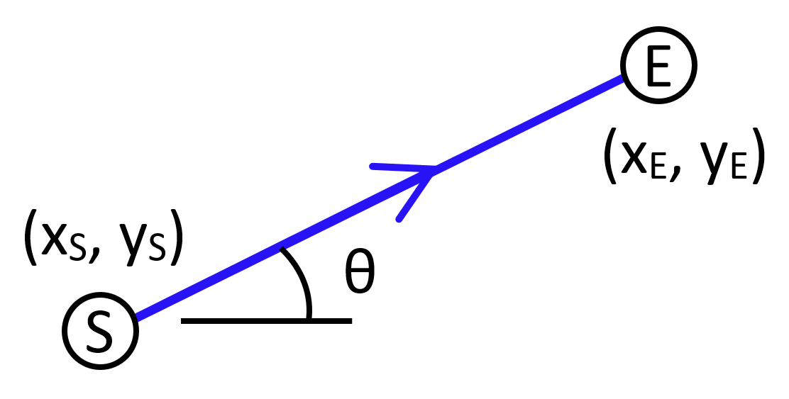
 Member rotation angle from horizontal
 Member direction
Figure 2: Generic member showing local coordinate system, orientation angle θ, length L, and global x-y coordinates
Member length (L):
\[ L = \sqrt{(x_E - x_S)^2 + (y_E - y_S)^2} \]
Where \( (x_S, y_S) \) and \( (x_E, y_E) \) are the coordinates of the start and end nodes, respectively.
Member orientation angle (θ):
\[ \theta = \arctan{\left( \frac{y_E - y_S}{x_E - x_S} \right)} \]
This angle is measured counterclockwise from the positive x-axis.
Direction cosines:
\[ c = \cos(\theta) = \frac{x_E - x_S}{L} \]
\[ s = \sin(\theta) = \frac{y_E - y_S}{L} \]
These values will be used repeatedly in forming the member stiffness matrices.
For example, for member 0:
\[ \theta_0 = \arctan{\left( \frac{2.5 - 0}{3 - 0} \right)} = 39.81^\circ \]
\[ c_0 = \cos(39.81^\circ) = 0.768 \]
\[ s_0 = \sin(39.81^\circ) = 0.640 \]
Step 2: Form Individual Member Stiffness Matrices
Each truss member has a stiffness matrix that relates the forces at its ends to the displacements at its ends. In the global coordinate system, a 2D truss member has 4 degrees of freedom (DOF): horizontal and vertical displacements at each end node.
The member stiffness matrix in global coordinates is:
| c2 | cs | -c2 | -cs |
| cs | s2 | -cs | -s2 |
| -c2 | -cs | c2 | cs |
| -cs | -s2 | cs | s2 |
Where:
- ki = Stiffness matrix for member i
- A = Cross-sectional area
- E = Elastic modulus
- L = Member length
- c = cos(θ)
- s = sin(θ)
The rows and columns correspond to DOFs in the order of horizontal and vertical stiffness components at the start node (S) and end node (E): \( [ S_x, S_y, E_x, E_y ] \).
For example, the stiffness matrix for member 0 is:
| 0.59 | 0.492 | -0.59 | -0.492 |
| 0.492 | 0.41 | -0.492 | -0.41 |
| -0.59 | -0.492 | 0.59 | 0.492 |
| -0.492 | -0.41 | 0.492 | 0.41 |
Step 3: Assemble the Global Structure Stiffness Matrix
The global stiffness matrix K combines all member stiffness matrices by summing contributions at each degree of freedom. For a truss with N nodes, K is a (2N × 2N) matrix.
Assembly process:
- Initialize K as a (2N × 2N) zero matrix
- For each member:
- Identify the global DOF indices for its start and end nodes
- Add the member's stiffness contributions to the appropriate positions in K
The global DOF numbering typically follows this pattern:
- Node 0: DOFs 0 (x-direction), 1 (y-direction)
- Node 1: DOFs 2 (x-direction), 3 (y-direction)
- Node i: DOFs 2i (x-direction), 2i+1 (y-direction)
For this example:
Only member 0 and member 4 connect to node 0, so the top left corner of the global stiffness matrix receives contributions from just these two members. We can use the above method to calculate the member stiffness matrices as:
| \( N_{0,x} \) | \( N_{0,y} \) | \( N_{1,x} \) | \( N_{1,y} \) | |
| \( N_{0,x} \) | 13150 | 10960 | -13150 | -10960 |
| \( N_{0,y} \) | 10960 | 9130 | -10960 | -9130 |
| \( N_{1,x} \) | -13150 | -10960 | 13150 | 10960 |
| \( N_{1,y} \) | -10960 | -9130 | 10960 | 9130 |
| \( N_{0,x} \) | \( N_{0,y} \) | \( N_{2,x} \) | \( N_{2,y} \) | |
| \( N_{0,x} \) | 10550 | 0 | -10550 | 0 |
| \( N_{0,y} \) | 0 | 0 | 0 | 0 |
| \( N_{2,x} \) | -10550 | 0 | 10550 | 0 |
| \( N_{2,y} \) | 0 | 0 | 0 | 0 |
Now, assembling these two members into an empty global stiffness matrix gives:
| \( N_{0,x} \) | \( N_{0,y} \) | \( N_{1,x} \) | \( N_{1,y} \) | \( N_{2,x} \) | \( N_{2,y} \) | \( N_{3,x} \) | ... | |
| \( N_{0,x} \) | 13150+10550 | 10960+0 | -13150 | -10960 | -10550 | 0 | - | ... |
| \( N_{0,y} \) | 10960+0 | 9130+0 | -10960 | -9130 | 0 | 0 | - | ... |
| \( N_{1,x} \) | -13150 | -10960 | 13150 | 10960 | - | - | - | ... |
| \( N_{1,y} \) | -10960 | -9130 | 10960 | 9130 | - | - | - | ... |
| \( N_{2,x} \) | -10550 | 0 | - | - | 10550 | 0 | - | ... |
| \( N_{2,y} \) | 0 | 0 | - | - | 0 | 0 | - | ... |
| \( N_{3,x} \) | - | - | - | - | - | - | - | ... |
| ... | ... | ... | ... | ... | ... | ... | ... | ... |
Global Stiffness Matrix K with only members 0 and 4 assembled
As we continue for all members and all nodes, we will obtain the full global stiffness matrix for this truss:
| 23690 | 10960 | -13150 | -10960 | -10550 | 0 | 0 | 0 | 0 | 0 | 0 | 0 | 0 | 0 |
| 10960 | 9130 | -10960 | -9130 | 0 | 0 | 0 | 0 | 0 | 0 | 0 | 0 | 0 | 0 |
| -13150 | -10960 | 33660 | 10140 | -4101 | 4101 | -16410 | -3281 | 0 | 0 | 0 | 0 | 0 | 0 |
| -10960 | -9130 | 10140 | 13890 | 4101 | -4101 | -3281 | -656.2 | 0 | 0 | 0 | 0 | 0 | 0 |
| -10550 | 0 | -4101 | 4101 | 28520 | -912.3 | -2278 | -3189 | -11600 | 0 | 0 | 0 | 0 | 0 |
| 0 | 0 | 4101 | -4101 | -912.3 | 8566 | -3189 | -4465 | 0 | 0 | 0 | 0 | 0 | 0 |
| 0 | 0 | -16410 | -3281 | -2278 | -3189 | 37370 | 0 | -2278 | 3189 | -16410 | 3281 | 0 | 0 |
| 0 | 0 | -3281 | -656.2 | -3189 | -4465 | 0 | 10240 | 3189 | -4465 | 3281 | -656.2 | 0 | 0 |
| 0 | 0 | 0 | 0 | -11600 | 0 | -2278 | 3189 | 28520 | 912.3 | -4101 | -4101 | -10550 | 0 |
| 0 | 0 | 0 | 0 | 0 | 0 | 3189 | -4465 | 912.3 | 8566 | -4101 | -4101 | 0 | 0 |
| 0 | 0 | 0 | 0 | 0 | 0 | -16410 | 3281 | -4101 | -4101 | 33660 | -10140 | -13150 | 10960 |
| 0 | 0 | 0 | 0 | 0 | 0 | 3281 | -656.2 | -4101 | -4101 | -10140 | 13890 | 10960 | -9130 |
| 0 | 0 | 0 | 0 | 0 | 0 | 0 | 0 | -10550 | 0 | -13150 | 10960 | 23690 | -10960 |
| 0 | 0 | 0 | 0 | 0 | 0 | 0 | 0 | 0 | 0 | 10960 | -9130 | -10960 | 9130 |
Global Structure Stiffness Matrix K
Step 4: Apply Boundary Conditions (Reduce the Stiffness Matrix)
Support conditions constrain certain DOFs to zero displacement. To solve for unknown displacements, we remove rows and columns corresponding to these constrained DOFs, creating the reduced stiffness matrix KR.
For example:
- Pin support: Both x and y displacements = 0 (remove 2 DOFs)
- Roller support (vertical): y displacement = 0 (remove 1 DOF)
- Roller support (horizontal): x displacement = 0 (remove 1 DOF)
In this example, we know that Node 0 is a pin support and Node 6 is a roller support in the vertical direction.
Therefore, both columns and rows can be removed from the global stiffness matrix K corresponding to \( N_{0,x} \), \( N_{0,y} \), and \( N_{6,y} \) to form the reduced stiffness matrix:
| 33660 | 10140 | -4101 | 4101 | -16410 | -3281 | 0 | 0 | 0 | 0 | 0 |
| 10140 | 13890 | 4101 | -4101 | -3281 | -656.2 | 0 | 0 | 0 | 0 | 0 |
| -4101 | 4101 | 28520 | -912.3 | -2278 | -3189 | -11600 | 0 | 0 | 0 | 0 |
| 4101 | -4101 | -912.3 | 8566 | -3189 | -4465 | 0 | 0 | 0 | 0 | 0 |
| -16410 | -3281 | -2278 | -3189 | 37370 | 0 | -2278 | 3189 | -16410 | 3281 | 0 |
| -3281 | -656.2 | -3189 | -4465 | 0 | 10240 | 3189 | -4465 | 3281 | -656.2 | 0 |
| 0 | 0 | -11600 | 0 | -2278 | 3189 | 28520 | 912.3 | -4101 | -4101 | -10550 |
| 0 | 0 | 0 | 0 | 3189 | -4465 | 912.3 | 8566 | -4101 | -4101 | 0 |
| 0 | 0 | 0 | 0 | -16410 | 3281 | -4101 | -4101 | 33660 | -10140 | -13150 |
| 0 | 0 | 0 | 0 | 3281 | -656.2 | -4101 | -4101 | -10140 | 13890 | 10960 |
| 0 | 0 | 0 | 0 | 0 | 0 | -10550 | 0 | -13150 | 10960 | 23690 |
Reduced Stiffness Matrix K_R
Step 5: Form the Reduced Load Vector
Similarly, create a load vector Q containing all applied forces at each DOF:
| \( N_{0,x} \) | \( N_{0,y} \) | \( N_{1,x} \) | \( N_{1,y} \) | \( N_{2,x} \) | \( N_{2,y} \) | \( N_{3,x} \) | \( N_{3,y} \) | \( N_{4,x} \) | \( N_{4,y} \) | \( N_{5,x} \) | \( N_{5,y} \) | \( N_{6,x} \) | \( N_{6,y} \) |
| 0 | 0 | 0 | -4 | 0 | 0 | 0 | -5 | 0 | 0 | 0 | -4 | 0 | 0 |
Complete Load Vector Q with DOF labels
Then form the reduced load vector QR by removing entries corresponding to constrained DOFs, just like we did for the stiffness matrix.
| 0 | -4 | 0 | 0 | 0 | -5 | 0 | 0 | 0 | -4 | 0 |
Step 6: Solve for Unknown Displacements
The fundamental stiffness equation relates forces to displacements:
\[ Q_R = K_R \cdot D_R \]Where DR is the vector of unknown displacements.
Now, solving for displacements:
\[ D_R = K_R^{-1} \cdot Q_R \]This requires inverting (or more commonly, performing LU decomposition or Cholesky decomposition on) the reduced stiffness matrix. Although this is computationally intensive when done by hand, it's straightforward to program on a computer using Matlab, Python, or any other language suited for matrix algebra.
Alternatively, the computation can be reduced further for hand calculations by partitioning the stiffness, force, and displacement matrices.
Displacement results:
The calculation of the reduced displacement vector results in displacements for all of the unknown degrees of freedom:
| 0.00140 | -0.00239 | 0.000740 | -0.00323 | 0.00113 | -0.00369 | 0.00153 | -0.00323 | 0.000871 | -0.00239 | 0.00227 |
By filling in the known 0-displacements at supports, we now know all node displacements in the system.
Node ID | Δx (ft) | Δy (ft) |
|---|---|---|
0 | 0 | 0 |
1 | 0.0014 | -0.00239 |
2 | 0.00074 | -0.00323 |
3 | 0.00113 | -0.00369 |
4 | 0.00153 | -0.00323 |
5 | 0.000871 | -0.00239 |
6 | 0.00227 | 0 |
Table 5: Nodal displacements in x and y directions
Step 7: Calculate Member Axial Forces
Once nodal displacements are known, individual member axial forces can be calculated using the transformation:
| -c | -s | c | s |
| \( Δ_{S,x} \) |
| \( Δ_{S,y} \) |
| \( Δ_{E,x} \) |
| \( Δ_{E,y} \) |
Where:
- qi = Axial force in member i (positive = tension, negative = compression)
- \( Δ_{S,x} \), \( Δ_{S,y} \) = Displacements at start node
- \( Δ_{E,x} \), \( Δ_{E,y} \) = Displacements at end node
For this example, the member axial force calculation for member 0 would be:
| -0.768 | -0.64 | 0.768 | 0.64 |
| 0 |
| 0 |
| 0.0014 |
| -0.00239 |
Complete member force results:
Repeating this calculation for all members gives us the axial forces in each member:
Member ID | Length (ft) | Axial Demand (kips) |
|---|---|---|
0 | 3.905 | -10.15 |
1 | 5.099 | -8.753 |
2 | 5.099 | -8.753 |
3 | 3.905 | -10.15 |
4 | 5.5 | 7.8 |
5 | 5 | 9.143 |
6 | 5.5 | 7.8 |
7 | 3.536 | 1.108 |
8 | 4.301 | -0.9626 |
9 | 4.301 | -0.9626 |
10 | 3.536 | 1.108 |
Table 6: Member axial forces for all members

Figure 3: Truss with members colored by force magnitude (scale in kips, tension positive)
Step 8: Calculate Support Reactions
Support reactions are found by multiplying the full stiffness matrix by the complete displacement vector (including zero displacements at supports):
\[ Q = K \cdot D \]
The reaction forces are the values of Q at the constrained DOFs. If there were applied loads at supports, subtract these to get the net reactions.
Support reaction results:
Node ID | Rx (kips) | Ry (kips) |
|---|---|---|
0 | 0 | 6.5 |
6 | 0 | 6.5 |
Table 7: Reaction forces at each support
Verification and Validation
After completing the analysis, always verify your results:
Static Equilibrium Check
Sum all forces (applied loads and reactions) in each direction:
\[ ΣF_x = 0 \]
\[ ΣF_y = 0 \]
\[ ΣM = 0 \]
Where M is the moment about any point in the structure.
If these don't sum to zero (within numerical tolerance), there's an error in the analysis.
Comparison with Hand Calculations
For simple, statically determinate trusses, compare member forces with results from the method of joints or method of sections.
Physical Reasonableness
- Do compression members make sense given the loading?
- Are displacement magnitudes reasonable?
- Do reactions point in expected directions?
Common Pitfalls and Tips
Sign Conventions
- Member forces: Positive = tension, negative = compression
- Displacements: Positive in the positive x or y direction
- Reactions: Report as positive when acting in the positive coordinate direction
Numerical Considerations
- Matrix conditioning: Very stiff members relative to flexible ones can cause numerical issues
- Units consistency: Ensure all units are consistent (e.g., all forces in kN, lengths in m, stress in MPa)
- Precision: Use sufficient numerical precision to avoid round-off errors in matrix operations
Modeling Tips
- Number nodes and members systematically
- Define member orientation consistently (though the method handles any orientation)
- Leverage symmetry when possible to reduce problem size
- Start with simplified models before adding complexity
Summary
The direct stiffness method provides a systematic, matrix-based approach to truss analysis that:
- Forms member stiffness matrices in global coordinates
- Assembles a global structure stiffness matrix
- Applies boundary conditions to reduce the system
- Solves for unknown displacements
- Calculates member forces and support reactions
This method is computationally efficient, handles complex structures naturally, and forms the basis for modern finite element analysis software. Mastering this technique is essential for any structural engineer working with analysis software or developing custom analysis tools.
Additional Resources
For more detailed examples and explanations of the stiffness method for truss analysis:
Try it yourself!
Visit trussanalysis.com to analyze your own truss structures using the direct stiffness method with our interactive calculator.
Keywords: truss analysis, direct stiffness method, matrix method, structural analysis, finite element method, displacement method, member forces, nodal displacements, stiffness matrix, structural engineering, matrix stiffness method, truss calculator, engineering tutorial, civil engineering, structural mechanics, FEA fundamentals